Using PRISM
Here, various different aspects of how the PRISM package can be used are described.
Minimal example
A minimal example on how to initialize and use the PRISM pipeline is shown here.
First, one has to import the Pipeline class and a ModelLink subclass:
>>> from prism import Pipeline
>>> from prism.modellink import GaussianLink
Normally, one would import a custom-made ModelLink subclass, but for this example one of the two ModelLink subclasses that come with the PRISM package is used (see Writing a ModelLink subclass for the basic structure of writing a custom ModelLink subclass).
Next, the ModelLink should be initialized, which is the GaussianLink class in this case.
In addition to user-defined arguments, every ModelLink subclass takes two optional arguments, model_parameters and model_data.
The use of either one will add the provided parameters/data to the default parameters/data defined in the class.
Since the GaussianLink class does not have default data defined, it is required to supply it with some data during initialization (using an array, dict or external file):
>>> # f(3) = 3.0 +- 0.1, f(5) = 5.0 +- 0.1, f(7) = 3.0 +- 0.1
>>> model_data = {3: [3.0, 0.1], 5: [5.0, 0.1], 7: [3.0, 0.1]}
>>> modellink_obj = GaussianLink(model_data=model_data)
Here, the GaussianLink class was initialized by giving it three custom data points and using its default parameters.
One can check this by looking at the representation of this GaussianLink object:
>>> modellink_obj
GaussianLink(model_parameters={'A1': [1.0, 10.0, 5.0], 'B1': [0.0, 10.0, 5.0],
                               'C1': [0.0, 5.0, 2.0]},
             model_data={7: [3.0, 0.1], 5: [5.0, 0.1], 3: [3.0, 0.1]})
The Pipeline class takes several optional arguments, which are mostly paths and the type of Emulator class that must be used.
It also takes one mandatory argument, which is an instance of the ModelLink subclass to use.
Since it has already been initialized above, the Pipeline class can be initialized:
>>> pipe = pipeline(modellink_obj)
>>> pipe
Pipeline(GaussianLink(model_parameters={'A1': [1.0, 10.0, 5.0], 'B1': [0.0, 10.0, 5.0],
                                        'C1': [0.0, 5.0, 2.0]},
                      model_data={7: [3.0, 0.1], 5: [5.0, 0.1], 3: [3.0, 0.1]}),
         working_dir='prism_0')
Since no working directory was provided to the Pipeline class and none already existed, it automatically created one (prism_0).
PRISM is now completely ready to start emulating the model.
The Pipeline allows for all steps in a full cycle (see PRISM pipeline) to be executed automatically:
>>> pipe.run()
which is equivalent to:
>>> pipe.construct(analyze=False)
>>> pipe.analyze()
>>> pipe.project()
This will construct the next iteration (first in this case) of the emulator, analyze it to check if it contains plausible regions and make projections of all active parameters.
The current state of the Pipeline object can be viewed by calling the details() method (called automatically after most user-methods), which gives an overview of many properties that the Pipeline object currently has.
This is all that is required to construct an emulator of the model of choice.
All user-methods, with one exception (evaluate()), solely take optional arguments and perform the operations that make the most sense given the current state of the Pipeline object if no arguments are given.
These arguments allow for one to modify the performed operations, like reconstructing/reanalyzing previous iterations, projecting specific parameters, evaluating the emulator and more.
Projections
After having made an emulator of a given model, PRISM can show the user the knowledge it has about the behavior of this model by making projections of the active parameters in a specific emulator iteration.
These projections are created by the project() method, which has many different properties and options.
For showing them below, the same emulator as the one in Minimal example is used.
Properties
Projections (and their figures) are made by analyzing a large set of evaluations samples.
For 3D projections, this set is made up of a grid of proj_res x proj_res samples for the plotted (active) parameters, where the values for the remaining parameters in every individual grid point are given by an LHD of proj_depth samples.
This gives the total number of analyzed samples as proj_res x proj_res x proj_depth.
Every sample in the sample set is then analyzed in the emulator, saving whether or not this sample is plausible and what the implausibility value at the first cut-off is (the first value in impl_cut).
This yields proj_depth results per grid point, which can be used to determine the fraction of samples that is plausible and the minimum implausibility value at the first cut-off in this point.
Doing this for the entire grid and interpolating them, creates a map of results that is independent of the values of the non-plotted parameters.
For 2D projections, it works the same way, except that only a single active parameter is plotted.
Note
When using a 2D model, the projection depth used to make a 2D projection will be proj_depth, which is to be expected.
However, when using an nD model, the projection depth of a 2D projection is equal to proj_res x proj_depth.
This is to make sure that for an nD model, the density of samples in a 2D projection is the same as in a 3D projection.
The project() method solely takes optional arguments.
Calling it without any arguments will produce six projection figures: three 2D projections and three 3D projections.
One of each type is shown below.
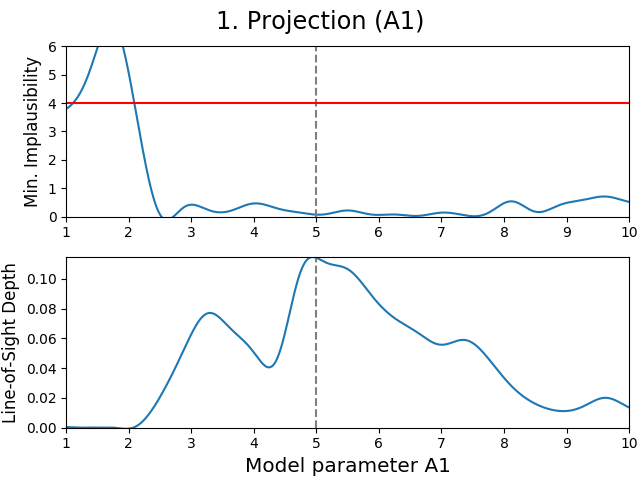
Fig. 3 2D projection figure of model parameter \(A_1\). The vertical dashed line shows the parameter estimate of \(A_1\), whereas the horizontal red line shows the first implausibility cut-off value.

Fig. 4 3D projection figure of model parameters \(A_1\) and \(B_1\). The dashed lines show the estimates of both parameters.
A projection figure is made up of two subplots. The upper subplot shows a map of minimum implausibility values that can be reached for any given value (combination) of the plotted parameter(s). The lower subplot gives a map of the fraction of samples that is plausible in a specified point on the grid (called “line-of-sight depth” due to the way it is calculated). Another way of describing this map is that it gives the probability that a parameter set with given plotted value(s) is plausible.
Both projection types have a different purpose. A 3D projection gives insight into what the dependencies (or correlations) are between the two plotted parameters, by showing where the best (top) and most (bottom) plausible samples can be found. On the other hand, a 2D projection is quite similar in meaning to a maximum likelihood optimization performed by MCMC methods, with the difference being that the projection is based on expectations rather than real model output. A combination of both subplots allows for many model properties to be derived, especially when they do not agree with each other.
Options
The project() method takes two (optional) arguments, emul_i and proj_par.
The first controls which emulator iteration should be used, while the latter provides the model parameters of which projections need to be made.
Since it only makes sense to make projections of active parameters, all passive parameters are filtered out of proj_par.
The remaining parameters are then used to determine which projections are required (which also depends on the requested projection types).
For example, if one wishes to only obtain projections of the \(A_1\) and \(B_1\) parameters (which are both active) in iteration 1, then this can be done with:
>>> pipe.project(1, ('A1', 'B1'))
This would generate the figures shown above, as well as the 2D projection figure of \(B_1\). By default, the last constructed emulator iteration and all model parameters are requested.
The remaining input arguments can only be given as keyword arguments, since they control many different aspects of the project() method.
The proj_type argument controls which projection types to make.
For 2D models, this is always ‘2D’ and cannot be modified.
However, for nD models, this can be set to ‘2D’ (only 2D projections), ‘3D’ (only 3D projections) or ‘both’ (both 2D and 3D projections).
By default, it is set to ‘both’.
The figure argument is a bool, that determines whether or not the projection figures should be created after calculating the projection data.
If True, the projection figures will be created and saved, which is done by default.
If False, the data that is contained within the projection figures will be calculated and returned in a dict.
This allows the user to either let PRISM create the projection figures using the standard template or create the figures themselves.
The align argument controls the alignment of the subplots in every projection figure. By default, it aligns the subplots in a column (‘col’), as shown in the figures above. Aligning the subplots in a row (‘row’) would give Fig. 3 as the figure below.
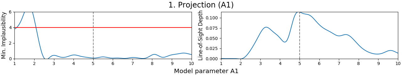
Fig. 5 2D projection figure of model parameter \(A_1\) with the ‘row’ alignment.
New in version 1.1.2: The show_cuts argument is also a bool, that determines whether to show all implausibility cut-off values in 2D projections (True) or only the first cut-off value (False, default).
In some cases, this may be useful when the first cut-off is not definitive in accepting or rejecting parameter values (as explained below for the smooth parameter).
The smooth argument is yet another bool, that determines what to do if a grid point in the projection figure contains no plausible samples, but does contain a minimum implausibility value below the first non-wildcard cut-off.
If False, which is the default, these values are kept in the figure, which may show up as artifact-like features.
If True, these values are set to the first cut-off, basically removing them from the projection figure.
This may however also remove interesting features.
Below are two identical projections, one that is smoothed and one that is not, to showcase this difference (these projections are from the second iteration, since this effect rarely occurs in the first iteration).
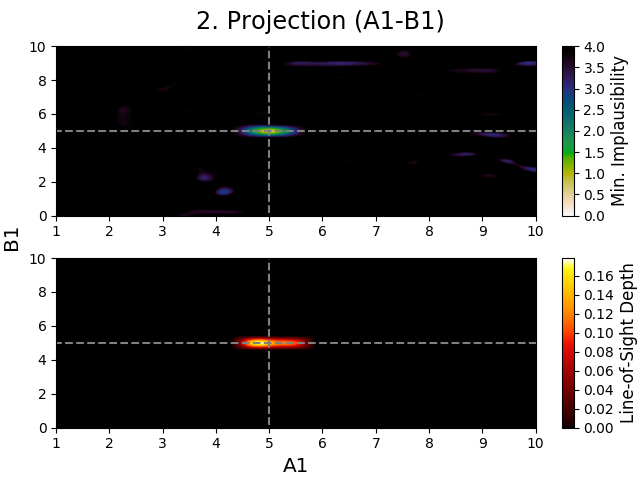
Fig. 6 Non-smoothed 3D projection figure of model parameters \(A_1\) and \(B_1\).
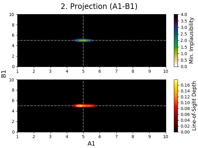
Fig. 7 Smoothed 3D projection figure of model parameters \(A_1\) and \(B_1\).
In these figures, one can see that the non-smoothed projection shows many features in the upper subplot that look like artifacts.
These features are however not artifacts, but caused by a sample (or samples) having its highest implausibility value being below the first implausibility cut-off, but still being implausible due to failing a later cut-off.
For example, if the implausibility cut-offs are [4.0, 3.7, 3.5] and a sample has implausibility values [3.9, 3.8, 3.2], it is found implausible due to failing to meet the second cut-off.
However, since the first value is still the highest implausibility value, that value is used in the projection figure.
Smoothing figures usually allows for 3D projections (2D projections rarely show this) to become less crowded, but they do throw away information.
It should therefore only be used when necessary.
The force argument is a bool, which controls what to do if a projection is requested for which data already exists.
If False (default), it will use the previously acquired projection data to create the projection figure if it does not exist, skip if it does or return the figure data if figure is False.
If True, the projection data and all associated projection figures will be deleted, and the projection will be recalculated.
The remaining seven arguments are keyword argument dicts, that need to be passed to the various different plotting functions that are used for creating the projection figures.
The fig_kwargs dict is passed to the figure() function when creating the projection figure instance.
The impl_kwargs_2D and los_kwargs_2D dicts are passed to the plot() function when making the minimum implausibility and line-of-sight depth subplots, respectively, for the 2D projections.
Similarly, the impl_kwargs_3D and los_kwargs_3D dicts are passed to the hexbin() function for 3D projections.
And, finally, the line_kwargs_est and line_kwargs_cut dicts are passed to the draw() function for drawing the parameter estimate and implausibility cut-off lines.
Dual nature (normal/worker mode)
PRISM features a high-level MPI implementation, as described in MPI implementation: all user-methods and most major methods are to be executed by all MPI ranks at the same time, and PRISM will automatically distribute the work among the available ranks within this function/method.
This allows for PRISM to be used with both serial and parallel models, by setting the MPI_call flag accordingly, while also allowing for the same code to be used in serial and parallel.
However, given that the emulator of PRISM can be very useful for usage in other routines, like Hybrid sampling, an external code will call PRISM’s methods.
In order to use PRISM in parallel with a parallelized model, this code would have to call PRISM with all MPI ranks simultaneously at all times, which may not always be possible (e.g., when using MCMC methods).
Therefore, PRISM has a dual execution/call nature, where it can be switched between two different modes.
In the default mode, PRISM works as described before, where all MPI ranks call the same user-code.
However, by using the WorkerMode context manager, accessed through worker_mode(), all code within will be executed in worker mode.
When in worker mode, all worker ranks are continously listening for calls from the controller rank, made with the _make_call() and _make_call_workers() methods.
They will continue to do so until the controller exits WorkerMode with __exit__().
Manually exiting should solely be done in advanced use-cases.
In worker_mode, one uses the following structure (assuming that the Pipeline instance is called pipe):
# Code to be executed in default mode

with pipe.worker_mode:
    if pipe.is_controller:
        # Code to be executed in worker mode

# More code to be executed in default mode
Note
All code that is inside the worker_mode context manager should solely be executed by the controller rank.
If not, all worker ranks will execute this code after the controller ranks exits the context manager.
Currently, it is not possible to make a context manager handle this automatically (the rejected PEP 377 describes this perfectly).
The _make_call() method accepts almost anything that can be called.
It can also be used when not in worker_mode, in which case it works the exact same way for all MPI ranks.
Its sole limitation is that all supplied arguments must be pickleable (e.g., compiled code objects are NOT pickleable due to safety reasons), both when used in worker_mode and outside of it.
The copyreg module can be used to register specific objects to become pickleable (including compiled code objects).
The worker_mode can be used in a variety of ways, as described below.
It can be used to access any attribute of the Pipeline instance:
with pipe.worker_mode:
    if pipe.is_controller:
        # Construct first emulator iteration
        pipe._make_call('construct', 1)

        # Print latest constructed emulator iteration
        print(pipe._make_call('emulator._get_emul_i', 1, 0))

        # Make a specific projection with the 'row' alignment
        pipe._make_call('project', 1, (0, 1), align='row')
which is equivalent to:
# Construct first emulator iteration
pipe.construct(1)

# Print latest constructed emulator iteration
print(pipe.emulator._get_emul_i(1, 0))

# Make a specific projection with the 'row' alignment
pipe.project(1, (0, 1), align='row')
The above two code snippets are equal to each other, and the worker_mode will most likely be used very rarely in this fashion.
However, by supplying the _make_call() method with a callable function (that can be pickled), externally defined functions can be executed:
# Enable worker mode
with pipe.worker_mode:
    if pipe.is_controller:
        # Import print function that prepends MPI rank to message
        from prism._internal import rprint

        # Make call to use this function
        # Equivalent to 'rprint("Reporting in.")'
        pipe._make_call(rprint, "Reporting in.")
This is especially useful when one combines a serial code with PRISM, but wants PRISM to execute in MPI. An application example of this is Hybrid sampling.
Changed in version 1.2.0: It is also possible to make a call that is solely executed by the workers, by using the _make_call_workers() method.
Changed in version 1.2.0: If any positional or keyword argument is a string written as ‘pipe.XXX’, it is assumed that ‘XXX’ refers to a Pipeline attribute of the MPI rank receiving the call.
It will be replaced with the corresponding attribute before exec_fn is called.
Changed in version 1.2.0: Initializing a worker mode within an already existing worker mode is possible and will function properly.
An example of this is using the construct() or crystal() method within worker mode, as both use one themselves as well.
Hybrid sampling
A common problem when using MCMC methods is that it can often take a very long time for MCMC to find its way on the posterior probability distribution function, which is often referred to as the burn-in phase.
This is because, when considering a parameter set, there is usually no prior information that this parameter set is (un)likely to result into a desirable model realization.
This means that such a parameter set must first be evaluated in the model before any probabilities can be calculated.
However, by constructing an emulator of the model, one can use it as an additional prior for the posterior probability calculation.
Therefore, although PRISM is primarily designed to make analyzing models much more efficient and accessible than normal MCMC methods, it is also very capable of enhancing them.
This process is called hybrid sampling, which can be performed easily with the utils module and will be explained below.
Note that an interactive version of this section can be found in the tutorials.
Algorithm
Hybrid sampling allows one to use PRISM to first analyze a model’s behavior, and later use the gathered information to speed up parameter estimations (by using the emulator as an additional prior in a Bayesian analysis). Hybrid sampling works in the following way:
- Whenever an MCMC walker proposes a new sample, it is first passed to the emulator of the model;
- If the sample is not within the defined parameter space, it automatically receives a prior probability of zero (or \(-\infty\) in case of logarithmic probabilities). Else, it will be evaluated in the emulator;
- If the sample is labeled as implausible by the emulator, it also receives a prior probability of zero. If it is plausible, the sample is evaluated in the same way as for normal sampling;
- Optionally, a scaled value of the first implausibility cut-off is used as an exploratory method by adding an additional (non-zero) prior probability. This can be enabled by using the impl_prior input argument for the
get_hybrid_lnpost_fn()function.
Since the emulator that PRISM makes of a model is not defined outside of the parameter space given by par_rng, the second step is necessary to make sure the results are valid.
There are several advantages of using hybrid sampling over normal sampling:
- Acceptable samples are guaranteed to be within plausible space;
- This in turn makes sure that the model is only evaluated for plausible samples, which heavily reduces the number of required evaluations;
- No burn-in phase is required, as the starting positions of the MCMC walkers are chosen to be in plausible space;
- As a consequence, varying the number of walkers tends to have a much lower negative impact on the convergence probability and speed;
- Samples with low implausibility values can optionally be favored.
Usage
In order to help the user with combining PRISM with MCMC to use hybrid sampling, the utils module provides two functions: get_walkers() and get_hybrid_lnpost_fn().
The get_walkers() function analyzes a set of proposed init_walkers and returns the positions that are plausible (and the number of positions that are plausible).
By default, it uses the available impl_sam of the last constructed iteration, but it can also be supplied with a custom set of proposed walkers or an integer stating how many proposed positions the function should check:
>>> # Use impl_sam if it is available
>>> n, p0 = get_walkers(pipe)

>>> # Request 2000 proposed samples
>>> n_walkers = 2000
>>> n, p0 = get_walkers(pipe, init_walkers=n_walkers)

>>> # Use custom init_walkers
>>> from e13tools.sampling import lhd
>>> init_walkers = lhd(n_walkers, pipe.modellink.n_par, pipe.modellink.par_rng)
>>> n, p0 = get_walkers(pipe, init_walkers=init_walkers)

>>> # Request 100 plausible starting positions (requires v1.1.4 or later)
>>> n, p0 = get_walkers(pipe, req_n_walkers=100)
As PRISM’s sampling methods operate in parameter space, the get_walkers() function automatically assumes that all starting positions are defined in parameter space.
However, as some sampling methods use unit space, normalized starting positions can be requested by setting the unit_space input argument to True.
One has to keep in mind that, because of the way the emulator works, there is no guarantee for a specific number of plausible starting positions to be obtained.
Having the desired emulator iteration already analyzed may give an indication how many starting positions in total need to be proposed to be left with a specific number.
Changed in version 1.2.0: It is now possible to request a specific number of plausible starting positions by using the req_n_walkers input argument. This will use a custom Metropolis-Hastings sampling algorithm to obtain the required number of starting positions, using the plausible samples in init_walkers as the start of every MCMC chain.
When the initial positions of the MCMC walkers have been determined, one can use them in an MCMC parameter estimation algorithm, avoiding the burn-in phase. This in itself can already be very useful, but it does not allow for hybrid sampling yet. Most MCMC methods require the definition of an lnpost() function, which takes a parameter set and returns the corresponding natural logarithm of the posterior probability. In order to do hybrid sampling, this lnpost() function must have the algorithm described above implemented.
The get_hybrid_lnpost_fn() function factory provides exactly that.
It takes a user-defined lnpost() function (as lnpost_fn) and a Pipeline object, and returns a function definition hybrid_lnpost(par_set, *args, **kwargs).
This hybrid_lnpost() function first analyzes a proposed par_set in the emulator, passes par_set (along with any additional arguments) to lnpost() if the sample is plausible, or returns \(-\infty\) if it is not.
The return-value of the lnpost() function is then returned by the hybrid_lnpost() function as well.
To make sure that the hybrid_lnpost() function can be used in both execution modes (see Dual nature (normal/worker mode)), all parallel calls to the Pipeline object are done with the _make_call() method.
The use of a function factory here allows for all input arguments to be validated once and then saved as local variables for the hybrid_lnpost() function.
Not only does this avoid that all arguments have to be provided and validated for every individual call, but it also ensures that the same arguments are used every time, as local variables of a function cannot be modified by anything.
Since users most likely use get_walkers() and get_hybrid_lnpost_fn() frequently together, the get_walkers() function allows for the lnpost_fn argument to be supplied to it.
This will automatically call the get_hybrid_lnpost_fn() function factory using the provided lnpost_fn and the same input arguments given to get_walkers(), and return the obtained hybrid_lnpost() function in addition to the starting positions of the MCMC walkers.
Application
Using the information above, using hybrid sampling on a model of choice can be done quite easily. For performing the MCMC analysis, we will be using the emcee package in this example.
Assume that we want to first analyze and then optimize the Gaussian model given by the GaussianLink class.
So, we first have to make an emulator of the model:
>>> from prism import Pipeline
>>> from prism.modellink import GaussianLink
>>> model_data = {3: [3.0, 0.1], 5: [5.0, 0.1], 7: [3.0, 0.1]}
>>> modellink_obj = GaussianLink(model_data=model_data)
>>> pipe = Pipeline(modellink_obj)
>>> pipe.construct()
Using the constructed emulator, we can perform a model parameter optimization using hybrid sampling. For this, we need to define an lnpost() function, for which we will use a simple Gaussian probability function:
def lnpost(par_set, pipe):
    # Create parameter dict for call_model
    par_dict = dict(zip(pipe.modellink.par_name, par_set))

    # Use wrapped model to obtain model output
    mod_out = pipe.modellink.call_model(pipe.emulator.emul_i,
                                        par_dict,
                                        pipe.modellink.data_idx)

    # Get the model and data variances
    # Since the value space is linear, the data error is centered
    md_var = pipe.modellink.get_md_var(pipe.emulator.emul_i,
                                       par_dict,
                                       pipe.modellink.data_idx)
    data_var = [err[0]**2 for err in pipe.modellink.data_err]

    # Calculate the posterior probability and return it
    sigma_2 = md_var+data_var
    diff = pipe.modellink.data_val-mod_out
    return(-0.5*(np.sum(diff**2/sigma2)))
Since the Pipeline object already has the model wrapped and linked, we used that to evaluate the model.
The GaussianLink class has a centered data error, therefore we can take the upper bound for every error when calculating the variance.
However, for more complex models, this is probably not true.
Next, we have to obtain the starting positions for the MCMC walkers. Since we want to do hybrid sampling, we can obtain the hybrid_lnpost() function at the same time as well:
>>> from prism.utils import get_walkers
>>> n, p0, hybrid_lnpost = get_walkers(pipe, unit_space=False,
                                       lnpost_fn=lnpost, impl_prior=True)
By setting impl_prior to True, we use the implausibility cut-off value as an additional prior.
Now we only still need the EnsembleSampler class and NumPy (for the lnpost() function):
>>> import numpy as np
>>> from emcee import EnsembleSampler
Now we have everything that is required to perform a hybrid sampling analysis.
In most cases, MCMC methods require to be executed on only a single MPI rank, so we will use the worker_mode:
# Activate worker mode
with pipe.worker_mode:
    if pipe.is_controller:
        # Create EnsembleSampler object
        sampler = EnsembleSampler(n, pipe.modellink.n_par,
                                  hybrid_lnpost, args=[pipe])

        # Run mcmc for 1000 iterations
        sampler.run_mcmc(p0, 1000)

        # Execute any custom operations here
        # For example, saving the chain data or plotting the results
And that is basically all that is required for using PRISM together with MCMC. For a normal MCMC approach, the same code can be used, except that one has to use lnpost() instead of hybrid_lnpost() (and, obtain the starting positions of the walkers in a different way).
General usage rules
Below is a list of general usage rules that apply to PRISM.
Unless specified otherwise in the documentation, any input argument in the PRISM package that accepts…
a bool (
True/False) also accepts 0/1 as a valid input;Noneindicates a default value or operation for obtaining this input argument. In most of these cases, the default value depends on the current state of the PRISM pipeline, and therefore a small operation is required for obtaining this value;Example
Providing
Nonetopot_active_par, where it indicates that all model parameters should be potentially active.the names of model parameters also accepts the internal indices of these model parameters. The index is the order in which the parameter names appear in the
par_namelist or as they appear in the output of thedetails()method;a parameter/sample set will accept a 1D/2D array-like or a dict of sample(s). As with the previous rule, the columns in an array-like are in the order in which the parameter names appear in the
par_namelist;a sequence of integers, floats and/or strings will accept (almost) any formatting including most special characters as separators as long as they do not have any meaning (like a dot for floats or valid escape sequences for strings). Keep in mind that providing
‘1e3’(or equivalent) will be converted to1000.0, as per Python standards;Example
- The following sequences are equal:
A, 1, 20.0, B;[A,1,2e1,B];“A 1 20. B”;“’[“ (A / }| \n; <1{}) ,,”>20.000000 !! \t< )?%\B ‘.
the path to a data file (PRISM parameters, model parameters, model data) will read in all the data from that file as a Python dict, with a colon
:acting as the separator between the key and value.
Depending on the used emulator type, state of loaded emulator and the PRISM parameter values, it is possible that providing values for certain PRISM parameters has no influence on the outcome of the pipeline. This can be either because they have non-changeable default values or are simply not used anywhere (given the current state of the pipeline);
All docstrings in PRISM are written in RST (reStructuredText) and are therefore best viewed in an editor that supports it (like Spyder);
All class attributes that hold data specific to an emulator iteration, start with index 1 instead of index 0. So, for example, to access the sample set that was used to construct iteration 1, one would use
pipe.emulator.sam_set[1](given that thePipelineobject is calledpipe).
External data files
When using PRISM, there are three different cases where the path to an external data file can be provided. As mentioned in General usage rules, all external files are read-in as a Python dict, with the colon being the separator between the key and value. Additionally, all lines are read as strings and converted back when assigned in memory, to allow for many different mark-ups to be used. Depending on which of the three files is read-in, the keys and values have different meanings. Here, the three different files are described.
PRISM parameters file
This file contains the non-default values that must be used for the PRISM parameters.
These parameters control various different functionalities of PRISM.
It is provided as the prism_par argument when initializing the Pipeline class and stored in the prism_dict property (a dict or array-like can be provided instead as well).
When certain parameters are set depends on their type:
- Emulator parameters: Whenever a new emulator is created;
- Pipeline parameters: When the
Pipelineclass is initialized;- Implausibility parameters: When the
analyze()method is called (saved to HDF5) or when an emulator iteration is loaded that has not been analyzed yet (not saved to HDF5);- Projection parameters: When the
project()method is called.
The default PRISM parameters file can be found in the prism/data folder and is shown below:
n_sam_init          : 500                   # Number of initial model evaluation samples
proj_res            : 25                    # Number of projected grid points per model parameter
proj_depth          : 250                   # Number of emulator evaluation samples per projected grid point
base_eval_sam       : 800                   # Base number for growth in number of model evaluation samples
sigma               : 0.8                   # Gaussian sigma/standard deviation (only required if method == 'gaussian')
l_corr              : 0.3                   # Gaussian correlation length(s)
impl_cut            : [0.0, 4.0, 3.8, 3.5]  # List of implausibility cut-off values
criterion           : None                  # Criterion for constructing LHDs
method              : 'full'                # Method used for constructing the emulator
use_regr_cov        : False                 # Use regression covariance
poly_order          : 3                     # Polynomial order for regression
n_cross_val         : 5                     # Number of cross-validations for regression
do_active_anal      : True                  # Perform active parameter analysis
freeze_active_par   : True                  # Active parameters always stay active
pot_active_par      : None                  # List of potentially active parameters
use_mock            : False                 # Use mock data
In this file, the key is the name of the parameter that needs to be changed, and the value what it needs to be changed to. PRISM itself does not require this default file, as all of the default values are hard-coded, and is therefore never read-in. An externally provided PRISM parameters file is only required to have the non-default values. The contents of this file is equal to providing the following as prism_par:
# As a dict
prism_par = {'n_sam_init': 500,
             'proj_res': 25,
             'proj_depth': 250,
             'base_eval_sam': 800,
             'sigma': 0.8,
             'l_corr': 0.3,
             'impl_cut': [0.0, 4.0, 3.8, 3.5],
             'criterion': None,
             'method': 'full',
             'use_regr_cov': False,
             'poly_order': 3,
             'n_cross_val': 5,
             'do_active_anal': True,
             'freeze_active_par': True,
             'pot_active_par': None,
             'use_mock': False}

# As an array_like
prism_par = [['n_sam_init', 500],
             ['proj_res', 25],
             ['proj_depth', 250],
             ['base_eval_sam', 800],
             ['sigma', 0.8],
             ['l_corr', 0.3],
             ['impl_cut', [0.0, 4.0, 3.8, 3.5]],
             ['criterion', None],
             ['method', 'full'],
             ['use_regr_cov', False],
             ['poly_order', 3],
             ['n_cross_val', 5],
             ['do_active_anal', True],
             ['freeze_active_par', True],
             ['pot_active_par', None],
             ['use_mock', False]]
Note that it is also possible to set any parameter besides Emulator parameters by using the corresponding class property.
Model parameters file
This file contains the non-default model parameters to use for a model.
It is provided as the model_parameters input argument when initializing the ModelLink subclass (a dict or array-like can be provided instead as well).
Keep in mind that the ModelLink subclass may not have default model parameters defined.
An example of the various different ways model parameter information can be provided is given below:
# name      : lower_bndry       upper_bndry     estimate
  A         : 1                 5               3
  Bravo     : 2                 7               None
  C42       : 3                 6.74
In this file, the key is the name of the model parameter and the value is a sequence of integers or floats, specifying the lower and upper boundaries of the parameter and, optionally, its estimate.
Similarly to the PRISM parameters, one can provide the following equivalent as model_parameters during initialization of a ModelLink subclass:
# As a dict
model_parameters = {'A': [1, 5, 3],
                    'Bravo': [2, 7, None],
                    'C42': [3, 6.74]}

# As an array_like
model_parameters = [['A', [1, 5, 3]],
                    ['Bravo', [2, 7, None]],
                    ['C42', [3, 6.74]]]

# As two array_likes zipped
model_parameters = zip(['A', 'Bravo', 'C42'],
                       [[1, 5, 3], [2, 7, None], [3, 6.74]])
Providing None as the parameter estimate or not providing it at all, implies that no parameter estimate (for the corresponding parameter) should be used in the projection figures.
If required, one can use the convert_parameters() function to validate their parameters formatting before using it to initialize a ModelLink subclass.
Model data file
This file contains the non-default model comparison data points to use for a model.
It is provided as the model_data input argument when initializing the ModelLink subclass (a dict or array-like can be provided instead as well).
Keep in mind that the ModelLink subclass may not have default model comparison data defined.
An example of the various different ways model comparison data information can be provided is given below:
# data_idx  : data_val          data_err        data_spc
  1, 2      : 1                 0.05    0.05    'lin'
  3.0       : 2                 0.05            'log'
  ['A']     : 3                 0.05    0.15
  1, A, 1.0 : 4                 0.05
Here, the key is the full sequence of the data identifier of a data point, where any character that is not a letter, number, minus/plus or period acts as a separator between the elements of the data identifier.
The corresponding value specifies the data value, data error(s) and data value space.
Braces, parentheses, brackets and many other characters can be used as mark-up in the data identifier, to make it easier for the user to find a suitable file lay-out.
A full list of all characters that can be used for this can be found in prism.aux_char_set and can be freely edited.
Similarly to the model parameters, the following is equal to the contents of this file:
# As a dict
model_data = {(1, 2): [1, 0.05, 0.05, 'lin'],
              3.0: [2, 0.05, 'log'],
              ('A'): [3, 0.05, 0.15],
              (1, 'A', 1.0): [4, 0.05]}

# As an array_like
model_data = [[(1, 2), [1, 0.05, 0.05, 'lin']],
              [3.0, [2, 0.05, 'log']],
              [('A'), [3, 0.05, 0.15]],
              [(1, 'A', 1.0), [4, 0.05]]]

# As two array_likes zipped
model_data = zip([(1, 2), 3.0, ('A'), (1, 'A', 1.0)],
                 [[1, 0.05, 0.05, 'lin'], [2, 0.05, 'log'], [3, 0.05, 0.15], [4, 0.05]])
It is necessary for the data value to be provided at all times.
The data error can be given as either a single value, where it assumed that the data point has a centered \(1\sigma\)-confidence interval, or as two values, where they describe the upper and lower bounds of the \(1\sigma\)-confidence interval.
The data value space can be given as a string or omitted, in which case it is assumed that the value space is linear.
Keep in mind that, as mentioned in Data identifiers (data_idx), providing a single element data identifier causes it to be saved as a scalar instead of a tuple.
Therefore, [‘A’] or (‘A’) is the same as ‘A’.
If required, one can use the convert_data() function to validate their data formatting before using it to initialize a ModelLink subclass.
Note
The parameter value bounds are given as [lower bound, upper bound], whereas the data errors are given as [upper error, lower error]. The reason for this is that, individually, the order for either makes the most sense. Together however, it may cause some confusion, so extra care needs to be taken.