The PRISM pipeline
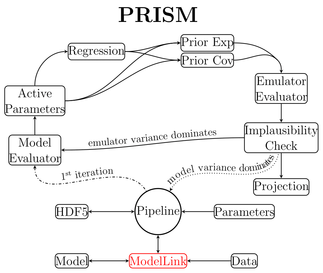
Fig. 1 The structure of the PRISM pipeline.
The overall structure of PRISM can be seen in Fig. 1 and will be discussed below.
The Pipeline object plays a key-role in the PRISM framework as it governs all other objects and orchestrates their communications and method calls.
It also performs the process of history matching and refocusing (see the PRISM paper for the methodology used in PRISM).
It is linked to the model by a user-written ModelLink object (see ModelLink: A crash course), allowing the Pipeline object to extract all necessary model information and call the model.
In order to ensure flexibility and clarity, the PRISM framework writes all of its data to one or several HDF5-files using h5py, as well as numpy.
The analysis of a provided model and the construction of the emulator systems for every output value, starts and ends with the Pipeline object.
When a new emulator is requested, the Pipeline object creates a large Latin-Hypercube design (LHD) of model evaluation samples to get the construction of the first iteration of the emulator systems started.
To ensure that the maximum amount of information can be obtained from evaluating these samples, a custom Latin-Hypercube sampling code was written.
This produces LHDs that attempt to satisfy both the maximin criterion as well as the correlation criterion.
This code is customizable through PRISM and publicly available in the e13Tools Python package.
This Latin-Hypercube design is then given to the Model Evaluator, which through the provided ModelLink object evaluates every sample.
Using the resulting model outputs, the Active Parameters for every emulator system (individual data point) can now be determined.
Next, depending on the user, polynomial functions will be constructed by performing an extensive Regression process for every emulator system, or this can be skipped in favor of a sole Gaussian analysis (faster, but less accurate).
No matter the choice, the emulator systems now have all the required information to be constructed, which is done by calculating the Prior Expectation and Prior Covariance values for all evaluated model samples (\(\mathrm{E}(D_i)\) and \(\mathrm{Var}(D_i)\)).
Afterward, the emulator systems are fully constructed and are ready to be evaluated and analyzed.
Depending on whether the user wants to prepare for the next emulator iteration or create a projection (see Projections), the Emulator Evaluator creates one or several LHDs of emulator evaluation samples, and evaluates them in all emulator systems, after which an Implausibility Check is carried out.
The samples that survive the check can then either be used to construct the new iteration of emulator systems by sending them to the Model Evaluator, or they can be analyzed further by performing a Projection.
The Pipeline object performs a single cycle by default (to allow for user-defined analysis algorithms), but can be easily set to continuously cycle.
In addition to the above, PRISM also features a high-level Message Passing Interface (MPI) implementation using the Python package mpi4py.
All emulator systems in PRISM can be constructed independently from each other, in any order, and only require to communicate when performing the implausibility cut-off checks during history matching.
Additionally, since different models and/or architectures require different amounts of computational resources, PRISM can run on any number of MPI processes (including a single one in serial to accommodate for OpenMP codes) and the same emulator can be used on a different number of MPI processes than it was constructed on (e.g., constructing an emulator using 8 MPI processes and reloading it with 6).
More details on the MPI implementation and its scaling can be found in MPI implementation.
In Using PRISM and ModelLink: A crash course, the various components of PRISM are described more extensively.
MPI implementation
Given that most scientific models are either already parallelized or could benefit from parallelization, we had to make sure that PRISM allows for both MPI and OpenMP coded models to be connected.
Additionally, since individual emulator systems in an emulator iteration are independent of each other, the extra CPUs required for the model should also be usable by the emulator.
For that reason, PRISM features a high-level MPI implementation for using MPI-coded models, while the Python package NumPy handles the OpenMP side.
A mixture of both is also possible (using the worker_mode context manager).
Here, we discuss the MPI scaling tests that were performed on PRISM.
For the tests, the same GaussianLink class was used as in Minimal example, but this time with \(32\) emulator systems (comparison data points) instead of \(3\).
In PRISM, all emulator systems are spread out over the available number of MPI processes as much as possible while also trying to balance the number of calculations performed per MPI process.
Since all emulator systems are stored in different HDF5-files, it is possible to reinitialize the Pipeline using the same Emulator class and ModelLink subclass on a different number of MPI processes.
To make sure that the results are not influenced by the variation in evaluation rates, we constructed an emulator of the Gaussian model and used the exact same emulator in every test.
The tests were carried out using any number of MPI processes between \(1\) and \(32\), and using a single OpenMP thread each time for consistency. We generated a Latin-Hypercube design of \(3\cdot10^6\) samples and measured the average evaluation rate of the emulator using the same Latin-Hypercube design each time. To take into account any variations in the evaluation rate caused by initializations, this test was performed \(20\) times. As a result, this Latin-Hypercube design was evaluated in the emulator a total of \(640\) times, giving an absolute total of \(1.92\cdot10^9\) emulator evaluations.
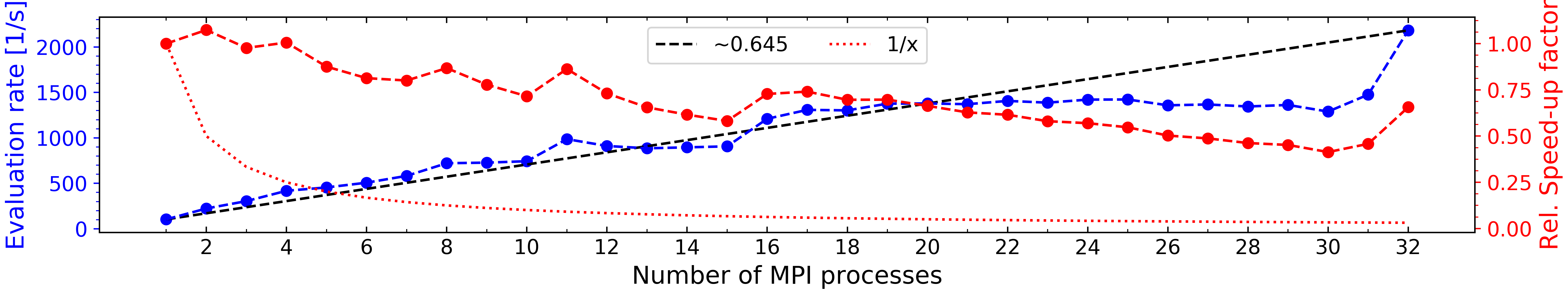
Fig. 2 Figure showing the MPI scaling of PRISM using the emulator of a simple Gaussian model with \(32\) emulator systems. The tests involved analyzing a Latin-Hypercube design of \(3\cdot10^6\) samples in the emulator, determining the average evaluation rate and executing this a total of \(20\) times using the same sample set every time. The emulator used for this was identical in every instance. Left axis: The average evaluation rate of the emulator vs. the number of MPI processes it is running on. Right axis: The relative speed-up factor vs. the number of MPI processes, which is defined as \(\frac{f(x)}{f(1)\cdot x}\) with \(f(x)\) the average evaluation rate and \(x\) the number of MPI processes. Dotted line: The minimum acceptable relative speed-up factor, which is always \(1/x\). Dashed line: A straight line with a slope of \({\sim}0.645\), connecting the lowest and highest evaluation rates. The tests were performed using the OzSTAR computing facility at the Swinburne University of Technology, Melbourne, Australia.
In Fig. 2, we show the results of the performed MPI scaling tests. On the left y-axis, the average evaluation rate vs. the number of MPI processes the test ran on is plotted, while the relative speed-up factor vs. the number of MPI processes is plotted on the right y-axis. The relative speed-up factor is defined as \(f(x)/(f(1)\cdot x)\) with \(f(x)\) the average evaluation rate and \(x\) the number of MPI processes. The ideal MPI scaling would correspond to a relative speed-up factor of unity for all \(x\).
In this figure, we can see the effect of the high-level MPI implementation. Because the emulator systems are spread out over the available MPI processes, the evaluation rate is mostly determined by the runtime of the MPI process with the highest number of systems assigned. Therefore, if the number of emulator systems (\(32\) in this case) cannot be divided by the number of available MPI processes, the speed gain is reduced, leading to the plateaus like the one between \(x=16\) and \(x=31\). Due to the emulator systems not being the same, their individual evaluation rates are different such that a different evaluation rate has a bigger effect on the average evaluation rate of the emulator the more MPI processes there are. This is shown by the straight dashed line drawn between \(f(1)\) and \(f(32)\), which has a slope of \({\sim}0.645\).
The relative speed-up factor shows the efficiency of every individual MPI process in a specific run, compared to using a single MPI process. This also shows the effect of the high-level MPI implementation, giving peaks when the maximum number of emulator systems per MPI process has decreased. The dotted line shows the minimum acceptable relative speed-up factor, which is always defined as \(1/x\). On this line, the average evaluation rate \(f(x)\) for any given number of MPI processes is always equal to \(f(1)\).